Chapter 2- expected utility
Risk Aversion in the expected utility approach
DefinitionThis obviously is equivalent to say that he does not want to take any risk with negative mean : indeed, if \(\widetilde{z}\) is a lottery with negative mean, then we have : \(\mathbb{E}\left[u(w+\widetilde{z})\right]=\mathbb{E}u(w+\mathbb{E}(\widetilde{z})+\widetilde{z}-\mathbb{E}(\widetilde{z}))\leq u(w+\mathbb{E}(\widetilde{z}))\leq u(w)\). A risk averse decision maker will hence accept to take a risk if the mean of the lottery is sufficiently large and positive.
We say that a decision maker is risk-averse if and only if he dislikes zero mean lotteries, that is he does not want to take a risk with zero mean : \(\forall\widetilde{x}\), s.t. \(\mathbb{E}(\widetilde{x})=0\), \(\forall w \: \mathbb{E}\left[u(w+\widetilde{x})\right]\leq u(w) \)
Risk aversion is linked to the concavity of \(u\).
Proposition
A decision maker is risk averse if and only if u is concave..
Proof. This can be easily shown by writing that the definition of risk aversion is equivalent to \(\forall\widetilde{y}, \mathbb{E}\left[u(\widetilde{y})\right]\leq u(\mathbb{E}(\widetilde{y}))\)
A risk averse individual is ready to pay to avoid a zero mean risk. The maximum amount he is ready to pay is called the risk-premium.
Risk Premium for a zero mean risk
DefinitionCertainty equivalent of a risk
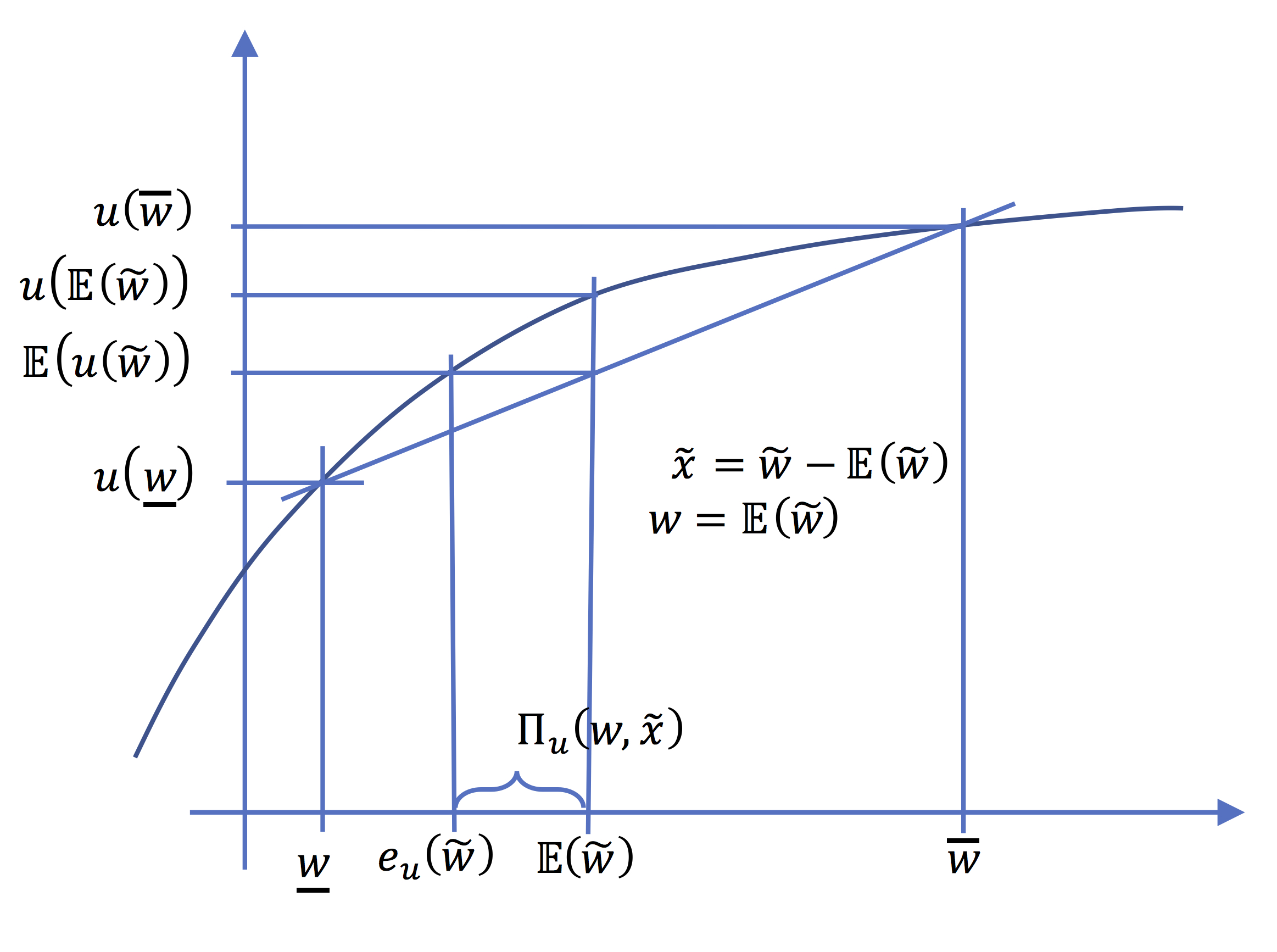
Given a zero mean risk, \(\widetilde{x}\), the risk premium \(\Pi_{u}(\widetilde{x})\) for a risk averse individual is defined by : \(\mathbb{E}\left[u(w+\widetilde{x})\right]=u(w-\Pi_{u}(\widetilde{x}))\)
For a given risk \(\widetilde{w}\) we can define the so-called "certainty equivalent". This is the sure income noted \(e_{u}(\widetilde{w})\) that gives the same level of utility as \(\widetilde{w}\).
Definition
The certainty equivalent \(e_{u}(\widetilde{w})\) of the random income \(\widetilde{w}\) for a risk averse individual is defined by : \(\mathbb{E}\left[u(\widetilde{w})\right]=u(e_{u}(\widetilde{w}))\). it is the sure income that gives the same expected utility.
The measure of risk aversion
The pupose of this section is to try to give a consistent definition to "more" or "less" risk aversion.2.1 Degrees of risk aversion
When can we say that a decision maker is "more risk averse" than another one? We know that a necessary condition for a risk to be accepted by a risk averse decision maker is that it has a strictly positive mean. A natural definition could then be :DefinitionTake two such individuals. Take the real (non decreasing) function \(\phi\) defined on the image of \(u\) (that is on \(u(\mathbb{R}))\), by \(\phi=v\circ u^{-1}\).
An invividual (entailed with a utility function \(v\)) is more risk averse than an individual (with a function \(u\)) if and only if, whenever \(u\) refuses a risk \(\widetilde{z}\), then \(v\) refuses too.\[\mathbb{E}(u(w+\widetilde{z})) <u(w)\Longrightarrow\mathbb{E}(v(w+\widetilde{z}))<v(w)\]
Take any random income \(\widetilde{z}\) , and set \(\widetilde{y}=u(w+\widetilde{z})\),
we have : \(\mathbb{E}v(w+\widetilde{z}))=\mathbb{E}\left[\phi(u(w+\widetilde{z}))\right]=\mathbb{E}\left[\phi(\widetilde{y})\right]\).
Suppose \(\mathbb{E}(u(w+\widetilde{z}))<u(w)\),
that is \(\mathbb{E}(\widetilde{y})<u(w)\).
Hence, because \(v\) is more risk averse, \(\mathbb{E}\left[\phi(\widetilde{y})\right]<\phi(u(w))\)
Hence the definition amounts to say :
\(\forall\widetilde{y}\) and \(c\) such that \(\mathbb{E}(\widetilde{y})<c\),then \( \mathbb{E}\left[\phi(\widetilde{y})\right]<\phi(c)\),
which implies thet \(\phi\) must be concave :
Indeed, if it were not the case there would exist \(\widetilde{y}_{0}\) such that \(\mathbb{E}\left[\phi(\widetilde{y}_{0})\right]>\phi(\mathbb{E}(\widetilde{y}_{0}))\), and then \(c\), such that \(\phi(\mathbb{E}(\widetilde{y}_{0}))<\phi(c)<\mathbb{E}\left[\phi(\widetilde{y}_{0})\right])\).
Conversely, if \(\phi=v\circ u^{-1}\) is concave, it is easy to see that \(v\) is more risk-averse than \(u\).
Proposition
An invividual (entailed with a utility function v) is more risk averse than an individual (with a function u) if and only if v is a concave transformation of u : \(v=\phi\circ u\), with \(\phi\) concave.
Proposition
If \(v\) is more risk averse than \u\) then \(\Pi_{v}(\widetilde{x})\geq\Pi_{u}(\widetilde{x})\) for all zero mean risk \(\widetilde{x}\).
\(v(w-\Pi_{v}(\widetilde{x}))=\phi\circ u(w-\Pi_{v}(\widetilde{x}))=\mathbb{E}\left[\phi\circ u(w+\widetilde{x})\right]\leq\phi\left[\mathbb{E}(u(w+\widetilde{x}))\right]=\phi(u(w-\Pi_{u}(\widetilde{x}))=v(w-\Pi_{u}(\widetilde{x}))\)
2.2 Differentiable case and index of absolute risk aversion
Suppose that \(u\) and \(v\) are twice continuously differentiable. In such a case concavity of \(u\) and \(v\) are equivalent to say that \(v"\) and \(u"\) are negative functions.
A direct calculus gives : \(v^{\prime}=(\phi^{\prime}\circ u)u^{\prime}\) and \(v^{\prime\prime}=(\phi^{\prime\prime}\circ u)(u^{\prime})^{2}+(\phi^{\prime}\circ u)u^{\prime\prime}\) that is \(\frac{-v^{\prime\prime}}{v^{\prime}}=\frac{-u^{\prime\prime}}{u^{\prime}}+\frac{-(\phi^{\prime\prime}\circ u)}{(\phi^{\prime}\circ u)}u^{\prime}\).
As (by concavity) \(\phi^{\prime\prime}\leq0\), \(\frac{-v^{\prime\prime}}{v^{\prime}}\geq\frac{-u^{\prime\prime}}{u^{\prime}}\). This motivates the following definition.
DefinitionWe have then :
For a decision maker entailed with a utility function \(u\), the Absolute Risk Aversion Index \(I_{u}(w)\) at the level of wealth \(w\) is defined by \[I_{u}(w)= \frac{-u^{\prime\prime}(w)}{u^{\prime}(w)}\]
Proposition
The following properties are equivalent
- (i) \(v\) is more risk averse than \(u\)
- (ii) \(v=\phi\circ u\), with \( \phi\) concave
- (iii) \(\Pi_{v}(\widetilde{x})\geq\Pi_{u}(\widetilde{x})\) for all zero mean risk \widetilde{x}
- (iv) \(\frac{-u^{\prime\prime}(w)}{u^{\prime}(w)}\leq\frac{-v^{\prime\prime}(w)}{v^{\prime}(w)}\), that is \(I_{u}(w)\leq I_{v}(w)\) for all \(w\), if we restrict to twice continuously differentiable functions.
We can link the above analysis with spectral risk indexes defined in the previous chapter. We defined, indeed, a spectral risk index \(U_{h}\) by : \[U_{h}(\widetilde{w})\equiv -\int_{a}^{b}h(x)F_{\widetilde{w}}(x)dx\]. In that definition \(h\), when non negative and non increasing, has been interpreted as the derivative \(u^{\prime}\) of the utility function \(u\) associated to a risk-averse decision maker. In that framework we can conclude that \(v\) is more risk-averse than \(u\) if : \[\frac{v'}{u'}\:\mathrm{non}\:\mathrm{increasing}\] This condition is more general than the condition on absolute risk aversion indexes.
2.3 Small risks and Arrow-Pratt approximation
It is interesting to examine the behaviour of risk premium for small risk and twice continuously differentiable functions \(u\). Fix a zero mean lottery \(\widetilde{x}\) and set \(\widetilde{y}=k\widetilde{x}\).The risk premium associated with \(\widetilde{y}\) is defined by \[\mathbb{E}\left[u(w+\widetilde{y})\right]=u(w-\Pi_{u}(\widetilde{y}))\].
For \( \widetilde{x}\) fixed we can examine the behaviour of the risk premium for small values of \(k\).
Set \(g(k)=\Pi_{u}(\widetilde{y})=\Pi_{u}(k\widetilde{x})\).
We have :
\[g(k)=g(0)+kg^{\prime}(0)+\frac{k^{2}}{2}g^{\prime\prime}(0)+o(k^{2})\].
Obviously \(g(0)=0\) : when there is no risk there is no risk premium!.
To compute \(g^{\prime}(0)\), we use an implicit function argument. Consider the identity \(\mathbb{E}\left[u(w+k\widetilde{x})\right]=u(w-g(k))\) which is true (by definition of the risk premium) for all \(k\).
Differentiating both sides with respect to \(k\) gives :
\[\mathbb{E}(\widetilde{x}u^{\prime}(w+k\widetilde{x}))=-g^{\prime}(k)u^{\prime}(w-g(k))\].
For \(k=0\) this gives \(\mathbb{E}(\widetilde{x})=-g^{\prime}(0)\).
As \(\mathbb{E}(\widetilde{x})=0\), this implies \(g^{\prime}(0)=0\).
Risk aversion is a second order phenomenon (for continuously differentiable functions). The risk premium is nul at a first order approximation.
Differentiating twice gives
\[\mathbb{E}(\widetilde{x}^{2}u^{\prime\prime}(w+k\widetilde{x}))=-g^{\prime\prime}(k)u^{\prime}(w-g(k))-(g^{\prime}(k))^{2}u^{\prime\prime}(w-g(k))\].
For \(k=0\) this gives
\[g^{\prime\prime}(0)=\frac{-u^{\prime\prime}(w)}{u^{\prime}(w)}\mathbb{E}(\widetilde{x}^{2})=I_{u}(w)\mathbb{E}(\widetilde{x}^{2})\]
Proposition
For a twice continuously differntiable function \(u\), the Arrow Pratt approximation of the risk premium is :\(\Pi_{u}(\widetilde{y})\sim\frac{1}{2}I_{u}(w) var(\widetilde{y})+o(var(\widetilde{y}))\)
Decreasing risk aversion
We are now interested in determining how the risk premium is affected by a change in initial wealth \(w\). The intuition, and some empirical evidences, seems to imply that wealthier people bear more easily risk than poorer. The risk premium for a given zero mean risk is decreasing with wealth. For all given w and zero mean risk \(\widetilde{x}\), The risk premium \(\Pi_{u}(\widetilde{x},w)\) verifies : \[\mathbb{E}(u(w+\widetilde{x}))=u(w-\Pi(\widetilde{x},w))\]Differentiating with respect to \(w\) gives : \[\mathbb{E}(u^{\prime}(w+\widetilde{x}))=u^{\prime}(w-\Pi_{u}(\widetilde{x},w))(1-\Pi_{w}^{\prime}(\widetilde{x},w))\], that gives : \[\Pi_{w}^{\prime}(\widetilde{x},w)u^{\prime}(w-\Pi_{u}(\widetilde{x},w))=u^{\prime}(w-\Pi_{u}(\widetilde{x},w))-E(u^{\prime}(w+\widetilde{x}))\].
This means that the risk premium is decreasing with \(w\) if (for all \(\widetilde{x}\) and \(w\)) : \[\mathbb{E}(-u^{\prime}(w+\widetilde{x}))\leq-u^{\prime}(w-\Pi_{u}(\widetilde{x},w))\].
As the function \(-u^{\prime}\) is increasing, this implies that \(-u^{\prime}\) is concave, i.e \(u^{\prime}\) convex.
Indeed \(-u^{\prime}(w-\Pi_{u}(\widetilde{x},w))\leq-u^{\prime}(w)=-u^{\prime}(E(w+x))\).
DefinitionThis definition is somewhat mysterious, but we shall see in the sequel that this indeed corresponds to a prudent behaviour.
We say that a risk-averse decision maker is "prudent" if u^{\prime} is a convex decreasing function.
Proposition
Only prudent decision makers have decreasing risk premium with initial wealth.
Proposition
The risk premium is decreasing with wealth if and only if the index of absolute risk aversion is decreasing with wealth.
Aversion for downside risk
Consider a variation of the problem of Sempronius. Suppose that the value itself of \(x\) (the foreign wealth) are not sure. For instance the prices are subject to variations due to changes in demand. The lottery \(\widetilde{y}_{1}\) is then defined in the following way : with probability \(\frac{1}{2}\) the boat perishes and the cargo is lost , \(y_{1}=w\) and with probability \(\frac{1}{2}\), when the boat succeeds, the wealth is (with equal probability) either \(w+x- \epsilon\) or \( w+x+\epsilon\). We have obviously\[\mathbb{E}(\widetilde{y}_{1})=\frac{1}{2}w+\frac{1}{2}(\frac{1}{2}(w+x-\epsilon)+\frac{1}{2}(w+x+\epsilon))=w+\frac{1}{2}x\]
Suppose now that the uncertainty (the noise) affects the bad state of nature. The lottery \(\widetilde{y}_{2}\), is such that with probability \(\frac{1}{2}\) the wealth is ether (with equal probability) \(w- \epsilon\) or \(w+ \epsilon\)., and with probability \(\frac{1}{2}\) it is equal to \( w+x\). We have also : \(\mathbb{E}(\widetilde{y}_{2})=w+\frac{1}{2}x\). It is easy to see that the variances are also identical : \(var(\widetilde{y}_{1})=var(\widetilde{y}_{2})\) .
The intution suggests that Sempronius would prefer the first one : he dislikes "downside" risk, that is risk beared by the bad states of nature. We have
\[\mathbb{E}(u(\widetilde{y}_{1})-\mathbb{E}(u(\widetilde{y}_{2}) = \frac{1}{2}\left(u(w)-\mathbb{E}\left(u(w+\widetilde{\epsilon})\right)\right)+\frac{1}{2}\left(\mathbb{E}\left(u(w+x+\widetilde{\epsilon})\right)-u(w+x)\right)\] \[= \frac{1}{2}\int\limits _{w}^{w+x}(u^{\prime}(s)-\mathbb{E}(u^{\prime}(s+\widetilde{\epsilon}))ds\]
\(\mathbb{E}(u(\widetilde{y}_{1})\geq\mathbb{E}(u(\widetilde{y}_{2})\)
for all \(x\) and \(w\) implies that for all \(s\) and all \(\epsilon\) , \[u^{\prime}(s)\geq\frac{u^{\prime}(s-\epsilon)+u^{\prime}(s+\epsilon)}{2}\].
With the same proof as for proposition 1, this is equivalent to \(u^{\prime}\) convex.
Proposition
A decision maker is averse for downside risk if and only if \(u^{\prime}\) is a decreasing positive and convex function.\par Prudence and downside risk aversion are equivallent concepts.
Classical utility functions
In this section we give some families of utility functions that are commonly used in Economics and Finance. Obviously, assuming that the decision maker has a specific utility function is rather restrictive. This is done to obtain tractable solutions to many problems. But we have to keep in mind that some of these are closely related to the choice of a narrow class of utility functions.
5.1 Quadratic
The first family is the quadratic set :DefinitionThis function gives for a lottery \(\widetilde{z}\): \[\mathbb{E}\left(u(\widetilde{z})\right)=\mathbb{E}(\widetilde{z})- \frac{1}{2a}\mathbb{E}(\widetilde{z}^{2})=\mathbb{E}(\widetilde{z})-\frac{1}{2a} \left(var(\widetilde{z})+\mathbb{E}(\widetilde{z})^{2}\right)\] That is : \[\mathbb{E}\left(u(\widetilde{z})\right)=u(\mathbb{E}\widetilde{z}))-\frac{1}{2a}var(\widetilde{z})\] which amounts to so called mean-variance models : for two lotteries having the same mean the decision maker will choose the one with the smaller variance. The main drawback of this kind of utility function is the fact that it does not fulfill the decreasing risk aversion hypothesis. Indeed : \[I_{u}(w)=\frac{1}{a-w}\] The eversion index is increasing with wealth. For this main reason, quadratic functions are prudently used to model decision behaviour in front of risk.
Quadratic function : \[u(w)=w-\frac{1}{2a}w^{2}\]
5.2 CARA (Constant absolute risk-aversion)
CARA functions are those for which \(I_{u}(w)\) is constant.DefinitionThis function is largely used for several reasons. One is very interesting. When the lottery \(\widetilde{z}\) is normally distributed with mean \(m\) and variance \(\sigma^{2}\), we have (proof let to the reader) : \[\mathbb{E}(u(\widetilde{z}))=u(m-\frac{1}{2}\rho\sigma^{2})\] That is to say that the risk premium is exactly \(\frac{1}{2}\rho\sigma^{2}\). The Arrow-Pratt Approximation is exact.
The family of CARA functions is the set of exponential function :\[u(w)=-\frac{1}{\rho}\exp(-\rho w)\]with \(\rho\geq0\).The index of absolute risk aversion is \(I_{u}(w)=\rho\), constant. It corresponds to "entropic risk measure" defined in the previous chapter.
5.3 Other harmonic absolute risk aversion functions.
We can easily obtain decrasing absolute risk aversion functions by taking \(I_{u}(w)=\frac{\beta}{w}\), for some \(\beta\geq0\). If we call \(w\times I_{u}(w)\) "the relative index of risk aversion" these functions are such that their relative index is constant. By doing so we define "Harmonic" Risk aversion functions. It is easy to see that that gives the following family.Definition
Constant relative risk aversion (CRRA) functions are defined by : \[u(w)=\frac{1}{1-\beta}w^{1-\beta}\] for \(\beta\neq1\) , and \[u(w)=\ln(w)\], for \(\beta=1\).