Chapter 1 - risk measure

Assumptions on Risk
Throughout this section we assume that the variable of interest is the income associated with a decision. It is customary to distinguish risky situations depending on the level of information the decision maker has on the possible values and on the probabilities of these values. The first wellknown dictinction, due to Knight in his work Risk, Uncertainty, and Profit, is between ”risk” and ”uncertainty”. ”Uncertainty must be taken in a sense radically distinct from the familiar notion of Risk, from which it has never been properly separated.... The essential fact is that risk means in some cases a quantity susceptible of measurement, ... It will appear that a measurable uncertainty, or risk proper, as we shall use the term, is so far different from an unmeasurable one...” We can classify ”uncertainty situations” as follows :
Definition
Uncertainty : There is radical uncertainty when the decision maker knows neither the events (possible values, consequences...) nor the probabilities of these. There is uncertainty when one knows the events (possible values, consequences...) but have no estimate (subjective or not) of the probabilities.
Whereas risky situations are those for which probabilities can be (more or less) defined.
Definition
We call risk the case when one knows the events (amounts) and have some estimate (subjective or objective) of the probability. Risk is said to be ambiguous when there is some uncertainty on the probability distribution.
Here, except in some circumstances, we describe risk through an underlying probabiliezd space \((\Omega,\mathcal{B},\mathbb{P})\). Income of the decision maker is then a real random variable defined on that space . For simplicity, we moreover assume, except when another assumption is mentioned, that the support of the studied random variables is bounded.In the sequel it will be represented by a real random variables which will be noted by a tilded letter such as \(\widetilde{w}\).
Assumption
The risk is represented by a random variable \(\widetilde{w}\) on \((\Omega,\mathcal{B},\mathbb{P})\)with support \(K\) compact (hence bounded) included in an open interval \(]a,b[\) :\[\Pr(\widetilde{w} \notin K) = 0\]
Such variables are hence essentially bounded and we note
\(\underline{w}\equiv \mathrm{ess-inf}(\widetilde{w})\) and \(\bar{w}\equiv \mathrm{ess-sup}(\widetilde{w})\)
We have \(a< \underline{w}\) and \(\bar{w} < b \)
Risk magnitude : cumulative distribution and quantile functions
2.1. (cumulative) Distribution Function
One of the usual ways to represent the risk is to draw up the histogram of frequencies of possible values or more generally density of probability: each possible value (or each range of values) i s associated with its frequency (its probability). A more general and satisfactory way consists in representing the distribution function (or cumulative distribution function). Set \(\widetilde{w}\) a random variable whose values belong to a closed interval included in \(\left]a,b\right[\). The distribution function gives the probability that the variable is less than a given threshold.
Definition
The distribution function \(F\) (CDF) of a real random variable \(\widetilde{w}\) is given by \[F(x)=\Pr \left[\widetilde{w}\leq x\right]\]. This function is increasing positive right continuous at any point \(\left[-\infty,+\infty\right]\) and such that \(x\leq a\Rightarrow F\left(x\right)=0\) and \(x\geq b\Rightarrow F\left(x\right)=1\)
A first question is "scope" of the risk. Such variable income is it more or less risky than another? The issue of risk measurement is an important question.
Distribution
We restrict our study to probability measures that are
mixtures of absolutely continuous distributions and discrete
ones. Discrete (jumps distribution functions) distributions as
in the first panel, absolutely continuous as in the second and
mixture asi n the third one of the figure.
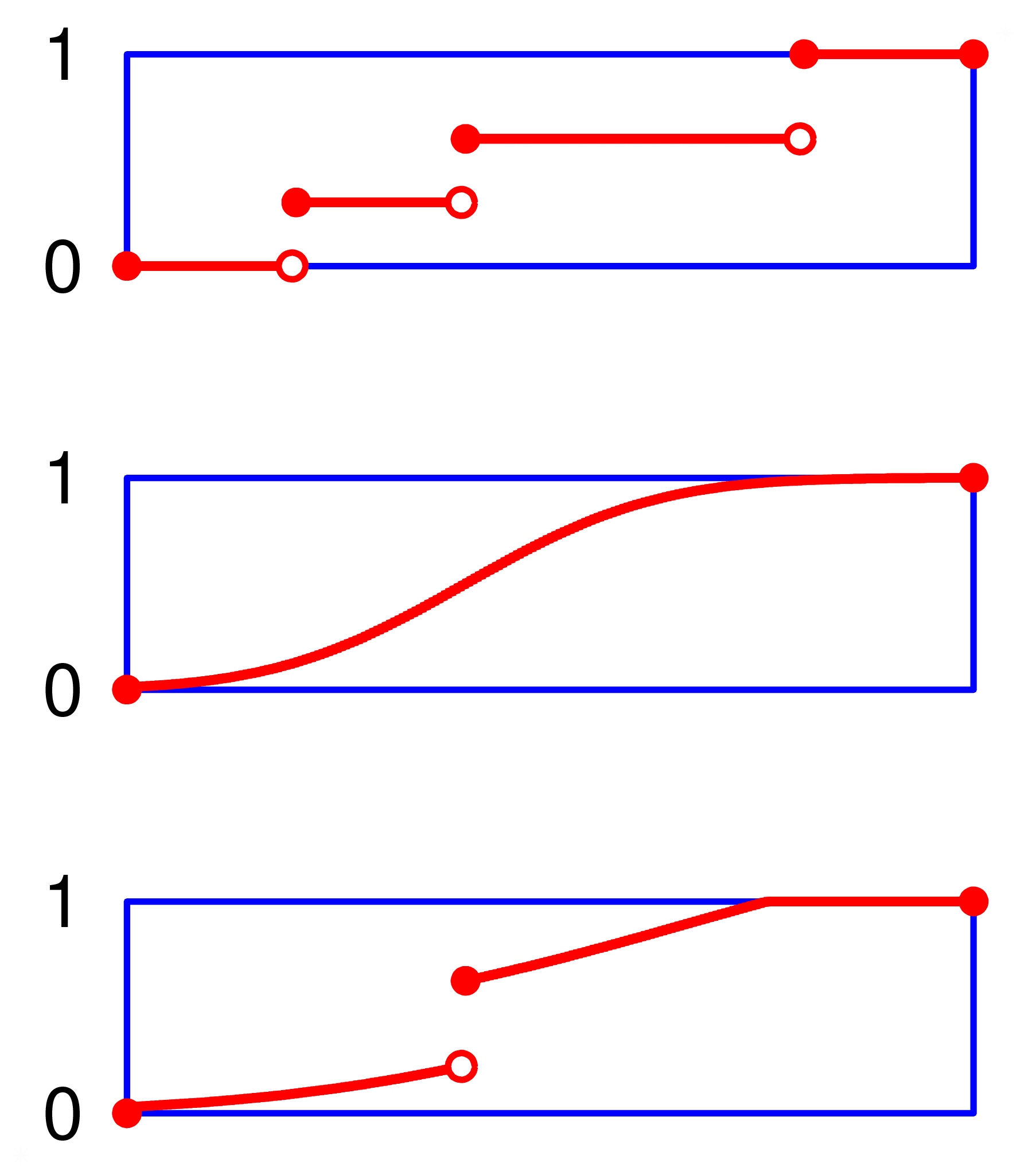
We exclude"singular distributions"as the one (the Cantor Distribution function) depicted in this figure. This distribution function, is continuous, but not absolutely continuous. It is almost everywhere differentiable, with a null derivative almost everywhere. It is obtained byputting the unit mass on the Cantor set.
Definition
Let two random variables \(\widetilde{v}\) and \(\widetilde{w}\) with support included in \(\left]a,b\right[\) . It is said that \(\widetilde{w}\) first-order stochastically dominates \(\widetilde{v}\), \(~\widetilde{w}\,\mathrm{FSD}\,\widetilde{v}\) , if \(\forall x,F_{\widetilde{w}}(x)\leq F_{\widetilde{v}}(x)\)
2.3. Quantile Function and Value at Risk
To that distribution function corresponds the quantile(s) function(s) or (generalized)inverse function(s). The lower quantile function will be useful here :
Definition
the (lower) quantile function is defined by: \[\alpha \in \left[0,1\right],\:F_{\tilde{w}}^{-1}(\alpha)=\inf\left\{ x\in[\underline{w},\bar{w}],F_{\tilde{w}}(x)\geq \alpha\right\} \] Note that \(F^{-1}\) is left continuous and that it could be equivalently defined by : \[\alpha \in \left[0,1\right],\:F_{\tilde{w}}^{-1}(\alpha)=\sup\left\{ x\in[\underline{w},\bar{w}],F_{\tilde{w}}(x)< \alpha\right\} \] .
Note that we have \(F^{-1}(0)=\underline{w}\) and \(F^{-1}(1)=\bar{w}<b\)
The quantile function reads as follows: in \(\alpha \times100\) percent of the cases, the variable is less than \(F_{\tilde{w}}^{-1}(\alpha)\).
Instead of lower quantile function one could have defined the upper quantile function : \[\alpha \in \left[0,1\right],\:\widehat{F}_{\tilde{w}}^{-1}(\alpha)=\inf\left\{ x\in[\underline{w},\bar{w}],F_{\tilde{w}}(x)> \alpha\right\} \] Note that \(\widehat{F}_{\tilde{w}}^{-1}\) is right continuous and \(\widehat{F}^{-1}\geq F^{-1}\). This upper quantile function will be more appropriate for random variables representing loss (see below).
The quantile function gives a first idea of the extent of the risk. In particular, it estimates the mattress to absorb losses (negative earnings) without using external inflows. For example we know that the random variable, hence the income, has a 10% probability to be less than \(F^{-1}(0.1)\) . So if the individual or institution has a reserve larger than \(-F^{-1}(0.1)\), bankruptcy probability is less than 0.1. Formally, if \(K\) is the reserve: \[\Pr\left(K+\widetilde{w}\leq0\right)<0.1\Rightarrow\Pr\left(\widetilde{w}\leq-K\right)<0.1 \Rightarrow-K\leq F^{-1}(0.1)\Rightarrow K\geq-F^{-1}(0.1)~\]. This remark leads to a first risk measure based on the quantile function.
Definition
If \(\widetilde{w}\) is the random income with quantile function \(F_{\tilde{w}}^{-1} \) , one calls Value at Risk at level \(\alpha \) : \[\mathrm{VaR}{}_{\widetilde{w}}(\alpha)=-F_{\widetilde{w}}^{-1}(\alpha)\] This is the needed reserve to absorb losses with at least probability \(1-\alpha\) .
Note that when the random variable is the loss (and not income), i.e. \(\widetilde{\ell}=-\widetilde{w}\) , then \(F_{\tilde{\ell}}(s)=1-F_{\widetilde{w}}(-s)\) and \(\mathrm{VaR}\) is: \[\mathrm{VaR}{}_{\widetilde{\ell}}(\alpha)=\widehat{F}_{\widetilde{\ell}}^{-1}(1-\alpha)~\].
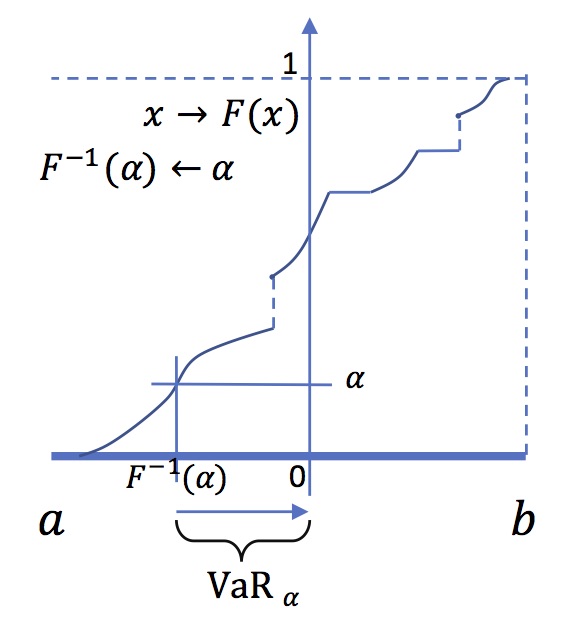
Value at risk
At level \(\alpha\) the value at risk is the opposite of the
quantile \(F^{-1}(\alpha)\). In this figure, the Value at risk
is positive.This means that a positive level of capital is
needed to reduce the probability of bankrupcy to \(\alpha\).
The risk measure associated to Value at Risk is obviously linked to first-order stochastic dominance :
Proposition
If \(\widetilde{w}\) first-order stochatically dominates \(\widetilde{v}\) , then \(\forall \alpha\in \left[0,1\right]\), \(\mathrm{VaR}{}_{\widetilde{w}}(\alpha)\leq \mathrm{VaR}{}_{\widetilde{v}}(\alpha)\)
Value at Risk is a "risk measure" very commonly used in practice, including, moreover, random variables of infinite support. For example, for a Gaussian random variable with mean \(\mu\) and variance \(\sigma^{2}\) , we have : \[F^{-1}(\alpha)=\mu+N^{-1}(\alpha)\sigma \] Where \(N^{-1}\) is the quantile function of the standard Gaussian distribution. For a Cauchy distribution the quantile function is : \[F^{-1}\left(\alpha\right)=\mu+\sigma\tan\left(\frac{\pi}{2}\left(2\alpha-1\right)\right)\] If the value at risk for a variable \(\widetilde{w}\) is smaller than that of \(\widetilde{v}\) that means that \(\widetilde{w}\) is more likely to be large than \(\widetilde{v}\). Big losses are less frequent with \(\widetilde{w}\). This is a first degree measure of risk.
Exercise 1
Give the quantile function of the exponential distibution \(\lambda \,e^{{-\lambda x}} \,1_{{x\geq 0}}\), of the uniform distribution \(\frac {1}{b-a} 1_{[a,b]}(x)\), and of the Bernouilli distribution \((\underline{w},p;\bar{w},(1-p))\)
Exercise 2
Assume \(\widetilde{w}\) distributed according to the exponential distribution on \([-D,+\infty]\),(\(D>0\)), \(dF(x)=\lambda \,,e^{{-\lambda (x+D)}}dx\).
Define \(\widetilde{z}=1_{[-D,C]}(\widetilde{w})\times\widetilde{w}\) where \(-D<C<0\).
- 1. Give the quantile function of \(\widetilde{w}\). Give the graphic representation of \(\int_{0}^{1}F^{-1}(t)dt\). Compute it.
- 2. Give the quantile function of \(\widetilde{z}\). (Hint : consider the "density" of \(\widetilde{z}\) compared to that of \(\widetilde{z}\) ; all the mass above \(C\) has been concentrated at 0); and then integrate to find \(F\)
Exercise 3
Explain the formula of \(\mathrm{VaR}\) when the variable is the loss \(\widetilde{\ell}=-\widetilde{w}\), using the "upper" quantile function
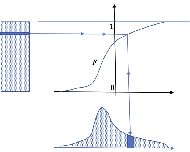
Quantile function and random simulation
Quantile function \(F^{-1}\) can be used to generate
random simulation of a variable whose CDF is \(F\) by the
mean of a uniformly distributed varable. Let \(U\) a
random variable uniformly distributed on \)[0,1]\), then
\(X\equiv F^{-1}(U)\) is distributed according to
\(F\).Indeed :\[\Pr(X\leq x)=\Pr(F^{-1}(U)\leq
x=\Pr(U\leq F(x))=F(x)\].
Imagine a vertical rectangular sand pile.each
slice of sand is projected horizontally through an oblique
sieve (whose shape is that of \(F\)) which sends it
vertically to another pile of sand so that the new pile
obtained is the desired density .
Risk measures based on the quantile function, the actuarial approach
In this section we are going to study risk measures that derive from the quantile function. Indeed the "shape of the quantile function give some information on risk.
First degree stochastic dominance does not compare "concentrations" of random variables, that is to which extend, the random variable is far from its mean. In this section we will try to give a meaning to the comparisons of concentrations.
3.1. Expected Shortfall
Some properties of the quantile function will allow us to analyze quite naturally the "concentration" of risks around the average. The first result is interesting:
PropositionThis result is obtained immediately,when \(F\) is strictly monotone and absolutely continuous, by change of variable \(x=F^{-1}(t)\text{ }\),\(dt=dF(x)\). It extends easily when \(F\) has jumps and flats.
If \(\widetilde{w}\) is a random variable with finite expected value (which is the case here, since its support is bounded) we have: \[\mathbb{E}\left(\widetilde{w}\right)=\int_{0}^{1}F^{-1}(t)dt\]
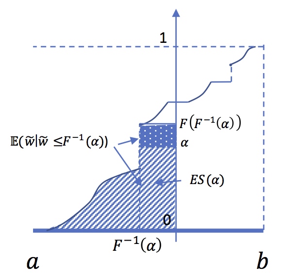
To better understand the risk we may be tempted to focus attention on the adverse event. For instance, we could evaluate the average income in the worst \(\alpha\) percents cases. When \(F^{-1}(\alpha)\) is not a point where mass is infinitely concentrated (not a jump of \(F\), i.e Dirac mass) then the average income in these unfavorable settings \( \widetilde{w}\leq F^{-1}(\alpha)\) , that is, \(\mathbb{E}(\widetilde{w}\mid\widetilde{w}\leq F^{-1}(\alpha))\),is equal to: \[\frac{1}{\alpha}\int_{0}^{\alpha}F^{-1}(t)dt\]
DefinitionWe see that ES is the average of the \(\mathrm{VaR}_{\widetilde{w}}(t)\) for \(t \leq \alpha\) . We will see later that we can generalize this kind of measure. In fact, the cumulative function of the quantile function gives an idea of the concentration of the probability distribution.
One calls "expected shortfall" (or \(\mathrm{aVaR}\), average value at risk, or \(\mathrm{cVaR}\), Conditional Value-at-Risk) at \(\alpha\) \[\mathrm{ES}{}_{\widetilde{w}}\left(u\right)=-\frac{1}{\alpha}\int_{0}^{\alpha}F^{-1}(t)dt\]
Expected Shortfall and Tail Conditional expectation at
level \( \alpha \)
It is tempting to consider the Tail Conditional
expectation : \( \mathbb{E} (\widetilde{w} \mid
\widetilde{w} \leq F^{-1}(\alpha))\).But this rises a
problem when \(F(F^{-1}(\alpha))>\alpha\), that is when
\(F^{-1}(\alpha))\) is a point where \(F\) has a jump.In
that case we have :
\[\int_{0}^{\alpha}F^{-1}(t)dt =
F(F^{-1}(\alpha))\mathbb{E}\left[\widetilde{w} \mid
\widetilde{w}\leq F^{-1}(\alpha)\right]\]
\[-\left[F(F^{-1}(\alpha))-\alpha\right]F^{-1}(\alpha)\]
3.2. Lorenz function
Definition
One calls absolute Lorenz function the function defined by: \[L_{\widetilde{w}}(\alpha)=\int_{0}^{\alpha}F^{-1}(t)dt.\]
In the same way, one can define the relative Lorenz curve as \(\ell_{\widetilde{w}}(\alpha)=\frac{1}{\alpha}L_{\widetilde{w}}(\alpha)\). When there is no jump at \(F^{-1}(\alpha)\), this is simply equal to \(\mathbb{E}(\widetilde{w}/\widetilde{w}\leq F^{-1}(\alpha))\), the expected income in quantile \(\alpha\).
Proposition
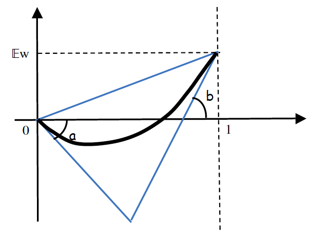
The Lorenz function \(L_{\widetilde{w}}\) associated to the random variable \(\widetilde{w}\) is a convex function (therefore continuous and left and right differentiable at each point) satisfying \(L_{\widetilde{w}}(0)=0,\:L_{\widetilde{w}}(1)=\mathbb{E}\left[\widetilde{w}\right]\) . The derivative (left and right) increases at any point, taking values between \(a\) and \(b\) . \(L'^{+}_{\widetilde{w}}(0)=\underline{w}\) and \(L'^{-}_{\widetilde{w}}(1)=\bar{w}\)
Conversely, every convex function \(L\) defined between 0 and 1, such that \(L(0)=0\), \(L(1)=c\) , with a slope greater than \(a\) at 0+ and less than \(b\) at 1 is in the Lorenz function of a real random variable with support included in \(\left]a,b\right[\) and with expected value equal to \(c\).
Lorenz curve
In this panel is represented the Lorenz curve for a random
variable taking values between \(a < 0\) and
\(b>0\).It lies in the triangle with slopes
\(a,\mathbb{E}(\widetilde{w}),b\)
3.3. Mean Preserving Spread
Given a random variable with support \(\left[a,b\right]\) , and expected value \(c=\mathbb{E}\left(\widetilde{w}\right)\) The position of the Lorenz curve in the triangle \(a\leq c\leq b\) gives a fairly accurate idea of the concentration. Consider for example the linear Lorenz function (thus the slope is \(c=\mathbb{E}\left(\widetilde{w}\right)) )\): \(L(u) \equiv cu \) . For that Lorenz function, \(F^{-1}\) is constant equal to \(c\) . The random variable is infinitely concentrated at \(c\) (Dirac mass) . The value is \(c\) with probability 1. In contrast consider the Lorenz curve formed by the two segments (with slope \(a\) and \(b\)), whose equation is \(L(u)=\max\left\{ au,-b(1-u)+c\right\}\) . This is the Lorenz function of the random variable with support \(\left[a,b\right]\) and expected value \(c\) which is the more "eccentric" since the only non-zero probability values are extreme values \(a \) and \(b\) .
In fact, when the Lorenz curve is far from the line \(c\times u\), that means that the random variable is less concentrated, and then more risky, around its mean \(c\). In the following is illustrated how to spread a distribution by the mean of mass transportation.
Elemental "mean-preserving spread" : mass
transportation
Take a distribution (here with density, ie absolutely
continuous). pick some mass out of an interval
\(\left[w_{1},w_{2}\right]\), and spread it outside,
taking care that the mean is preserved. It is just as if
you take some sand out of the middle of a sand pile, but
leaving the center of inertia in the same position. Take
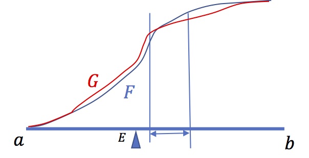
then the new CDF \(G\), If \(F\) is the original one, then
\[w\le w_{1}\Rightarrow G(w)\geq F(w)\] and \[w\geq
w_{2}\Rightarrow G(w)\leq F(w)\].In
\(\left[(w_{1},w_{2}\right]\), \(G-F\) is decreasing, So
that There exists a unique \(\widehat{w}\) such that
\[w\leq \widehat{w} \Rightarrow G(w)\geq F(w)\] and
\[w\geq \widehat{w} \Rightarrow G(w)\leq F(w)\]. Take
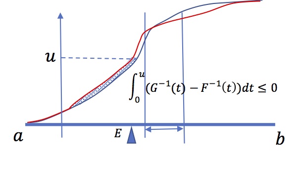
\(H(\alpha)\equiv\int_{0}^{\alpha}(G^{-1}(t)-F^{-1}(t))dt\).
We have \(H(0)=0 \) and (because the two variables have
the same mean, \(H(1)=0\). From above we know there exists
a quantile \(\widehat{\alpha}=F(\widehat{w})\) such that :
\[\alpha \leq \widehat{\alpha} \Rightarrow
H'(\alpha)=G^{-1}(\alpha)-F^{-1}(\alpha)\leq 0 \] and
\[\alpha \geq \widehat{\alpha} \Rightarrow
H'(\alpha)=G^{-1}(\alpha)-F^{-1}(\alpha)\geq 0\]
\(H\) is decreasing on the left of \(\widehat{\alpha}\),
and increasing on the right. This implies that \(H\) is
always negative.
We conclude that the Lorenz curve of the second variable is below the one of the first
Definition
Given two random variables \(\widetilde{v}\) and \(\widetilde{w}\) with support included in \(\left]a,b\right[\) and with the same mean. It is said that \(\widetilde{v}\) is less concentrated than, or more risky than, or a mean preserving spread of \(\widetilde{w}\) , That we note : \[\widetilde{w}\succsim\widetilde{v}\] if we can get the distribution of \(\widetilde{v}\) by the mean of a sequence (possibly infinite) of elemental mean-preserving spreads of \(\widetilde{w}\).
We have then the following result
Proposition
Given two random variables \(\widetilde{v}\) and \(\widetilde{w}\) with support included in \(\left]a,b\right[\) and with the same mean, then : \[\widetilde{w}\succsim\widetilde{v}\Longleftrightarrow\forall \alpha\in[0,1],L_{\widetilde{v}}\left(\alpha\right)\leq L_{\widetilde{w}}\left(\alpha\right)\]
Exercise 1
Give the Lorenz function of the exponential distibution \(\lambda \,e^{{-\lambda x}} \,1_{{x\geq 0}}\), of the uniform distribution \(\frac {1}{b-a} 1_{[a,b]}(x)\), and of the Bernouilli distribution \((\underline{w},p;\bar{w},(1-p))\)
Exercise 2
Why the Lorenz function of the Cauchy distribution does not exist?
Exercise 3
Study the link betwwen (relative) Lorenz curve and Gini index and the dispersion of values by lookin at this text
3.4. Generalized "\(\mathrm{aVaR}\)" : spectral preference criterions, spectral measures.
The aim of a risk measure is to define a numerical criterion associated to a random income designed to compare risky situations and take decisions. it is implicitely linked to some assumptions on the decision maker attitude towerds risk. For instance, if we assume (and it is natural to do so) that the decision maker prefers high incomes to low ones, then if \(\widetilde{w}\) stochastically dominates at the first order \(\widetilde{v}\), he will undoubtfully prefer \(\widetilde{w}\). In that situation all the values at risk at any threshold are smaller for \(\widetilde{w}\). Unfortunately, this criterion is very poor, since it allows to compare only variables whose quantile functions don't cross. We hence need to define measures that are able to compare any pair of random variables.
In the sequel we study decision criterions that are either "risk measures" as described in the litterature (indexes that are big when "risk" is big essentially aimed at defining the size of reserves to avoid bankrupcy) or "preference criterions" (indexes that allow to compare two random incomes and tell which one is better). This latter approach is tightly linked to models of behaviour in front of risk. From now if \(U\) is a preference criterion, then \(-U\) can be considered as a risk measure.
The idea developped in this paragraph is to use a linear transformation (linear form) of the quantile function. But this will necessary lead to make some other assumption about the attitude towards spread.
Definition : spectral preference criterion
Let \(\varphi\) an integrable real function defined on \(\left[0,1\right]~\) . Define (so called spectral preference criterion) :\[R_{\varphi}\left(\widetilde{v}\right)\equiv\int_{0}^{1}\varphi(t)F_{\widetilde{v}}^{-1}(t)dt\] If we normalize \(\varphi\) such that \(\int_{0}^{1}\varphi(t)dt=1\), \(R_{\varphi}\) is a weighted average of \(F^{-1}\), i.e (opposite of) Values at Risks \(\rho_{\varphi}\equiv -R_{\varphi}\) is the correspondent "spectral risk measure"
The first remark is simple.If \(\varphi\) is positive, if \(\widetilde{w} \: \mathrm{FSD} \widetilde{v}\) then \(R_{\varphi}(\widetilde{w})\geq R_{\varphi}(\widetilde{v})\) . In fact the one can derive the following proposition
Proposition (FSD)
Given two random variables \(\widetilde{v}\) and \(\widetilde{w}\) with support included in \(\left]a,b\right[\), (i),(ii),(iii) and (iv) are equivallent :
- (i) \(\widetilde{w} \:\mathrm{FSD}\:\widetilde{v}\)
- (ii) \(\forall \alpha\in [0,1],F_{\widetilde{w}}^{-1}(\alpha)\geq F_{\widetilde{v}}^{-1}(\alpha)\)
- (iii )\(\forall \alpha\in [0,1],\mathrm{VaR}_{\widetilde{w}}(\alpha)\leq\mathrm{VaR}_{\widetilde{v}}(\alpha)\)
- (iv) \(\forall\varphi\:\mathrm{positive},\:R_{\varphi}\left(\widetilde{w}\right)\geq R_{\varphi}\left(\widetilde{v}\right)\)
A spectral preference criterion based on positive weight function \(\varphi\) is an index that concerns first order of stochastic dominance, that is likelyhood of "large values". It does not take into account concentration or dispersion around the mean. We have seen that, precisely, the Lorenz function gives that kind of information. Assume that \(\varphi\) is right continuous non-increasing on \([0,1]\). Define the positive measure \(\eta\) by \(d\eta(\alpha)=-d\varphi(\alpha)\) . Replacing in the expression of \(R_{\varphi}\) yields:
\[R_{\varphi} (\widetilde{v}
)=\int_{0}^{1}\left[\varphi(1)+\int_{t}^{1} d\eta(s)
\right]F_{\widetilde{v}}^{-1}(t)dt
=\varphi(1)\mathbb{E}(\widetilde{v})+
\int_{0}^{1}\int_{0}^{1}\mathrm{1}_{[t,1]}(s)F^{-1}(t)d\eta(s)dt\]
\[R_{\varphi} (\widetilde{v}
)=\varphi(1)\mathbb{E}(\widetilde{v})+
\int_{0}^{1}\int_{0}^{1}\mathrm{1}_{[0,s]}(t)F^{-1}(t)dtd\eta(s)
=\varphi(1)\mathbb{E}(\widetilde{v})+
\int_{0}^{1}L_{\widetilde{v}}(s) d\eta(s)\]
Thus, for two random variables with the same mean:
\[R_{\varphi}(\widetilde{w})-R_{\varphi}(\widetilde{v})
=\int_{0}^{1}\left\{L_{\widetilde{w}}(\alpha)
-L_{\widetilde{v}}(\alpha)\right\}d\eta(\alpha)~\]
So we can deduce that when \(\varphi\) is a non increasing
right continuous function : \[\widetilde{w}\succsim\widetilde{v}\Longrightarrow
R_{\varphi}\left(\widetilde{w}\right)\geq
R_{\varphi}\left(\widetilde{v}\right)\]
Conversely, if for all \(\varphi\) non increasing right continuous function on \([0,1]\), \(R_{\varphi}\left(\widetilde{w}\right)\geq R_{\varphi}\left(\widetilde{v}\right)\), then we must have \(\forall \alpha\in [0,1], L_{\widetilde{v}}\left(\alpha \right)\leq L_{\widetilde{w}}\left(\alpha\right)\) . We can thus state
Proposition
Given two random variables \(\widetilde{v}\) and \(\widetilde{w}\) with support included in \(\left]a,b\right[\) and the same mean. Then (i),(ii),(iii),(iv) are equivalent :
- (i)\(\widetilde{w}\succsim\widetilde{v}\)
- (ii) \( \forall \alpha\in [0,1],L_{\widetilde{w}}(\alpha)\geq L_{\widetilde{v}}(\alpha)\)
- (iii) \(\forall \alpha\in [0,1],\mathrm{ES}_{\widetilde{v}}(\alpha)\geq\mathrm{ES}_{\widetilde{w}}(\alpha)\)
- (iv)\(\forall\varphi\:\mathrm{non \:increasing\:right\:continuous\:on\:[0,1]},\:R_{\varphi}\left(\widetilde{w}\right)\geq R_{\varphi}\left(\widetilde{v}\right)\)
When \(\varphi\) is non increasing, \(R_{\varphi}\left(\widetilde{w}\right)\) can thus be regarded as a "measure" of the concentration risk of \(\widetilde{w}\) . When ones takes for example \(\varphi(t)\equiv \frac{1}{\alpha}1_{\left[0,\alpha\right]}(t)\) , which is a non increasing normalized step function, \(-R_{\varphi}\left(\widetilde{w}\right)\) is then just the expected shortfall at the level \(\alpha\) .
3.5. Distorsion (or Wang) criterions and rank dependent expected value model
3.5.1. Distortion criterions
The previous criterion is tightly linked to what is called distorsion (or Wang) measures and "rank dependent expected value" or " Yaari's dual criterion". Consider the following spectral criterion : \[R_{\varphi}\left(\widetilde{w}\right)=\int_{0}^{1}\varphi(t)F_{\widetilde{w}}^{-1}(t)dt\] where \(\varphi\) is a given positive real, integrable function such that \(\int_{0}^{1}\varphi(t)dt=1\). Consider that the underlying probability space is \(\Omega=\left[0,1\right]\) with uniform probability distribution \(d\mathbb{P}(\omega)=d\omega\). Under that condition \(W(\omega)\equiv F_{\widetilde{w}}^{-1}(\omega)\) is a random variable with the same law as \(\widetilde{w}\). We can rewrite \(R_{\varphi}\left(\widetilde{v}\right)\) : \[R_{\varphi}\left(\widetilde{w}\right)=\int_{\Omega}W(\omega)d\mathbb{Q}(\omega)\] Where \(d\mathbb{Q}(\omega)=\varphi(\omega)d\omega\) This is the expected value of \(W\) under a "distorded" probability distribution.
Another way to find the same result can be obtained in the particular case where \(F_{w}\) is continuous and strictly increasing. Indeed changing variable \(x=F_{\widetilde{w}}^{-1}(t)\) : \[R_{\varphi}\left(\widetilde{w}\right)=\int_{a}^{b}x\varphi(F_{\widetilde{w}}\left(x\right))dF_{\widetilde{w}}(x)\] Taking \(\phi(\alpha)\equiv\int_{0}^{\alpha}\varphi(t)dt\) and \(\phi\left(F(x)\right)\equiv\psi\left(x\right)\) : \[R_{\varphi}\left(\widetilde{w}\right)=\int_{a}^{b}xd\psi(x)\] As moreover we have \(\phi\left(1\right)=1\) this amounts to replace the distribution \(F\) by the distorted distribution \(\psi\) and take the expected value.
More generally we could have defined some generalized spectral criterion. Instead of a (positive) function \(\varphi\) one can generalize and take a probability distribution on \([0,1]\) (with possibly a Dirac masses) characterizd by a right continuous increasing cumulative distribution function \(\phi\), with \(\phi(1)=1\) . A natural generalization consists in defining the criterion \(S_{\phi}\) by : \[S_{\phi}(\widetilde{w})=\int_{0}^{1}F^{-1}_{\widetilde{w}}(t)d\phi(t)\] Note that, since random variables are bounded, \(\phi\) can have a jump (Dirac mass) at 0 or 1 . So that the above (Stieljes) integral must be taken from \(0^{-}\) to \(1^{+}\).
This lead to the definition :
Definition
The Wang or "distorsion criterion" associated to the distorsion function \(\phi\) non decreasing, right continuous from \([0,1]\) to \([0,1]\) with \(\phi(1)=1\) is defined by : \[S_{\phi}(\widetilde{w})=\int_{0}^{1}F^{-1}_{\widetilde{w}}(t)d\phi(t)\] (The (Stieljes) integral above taken between \(0^{-}\) and \(1^{+}\))
This criterion generalizes spectral criterions with positive spectral function \(\varphi\).
Concavity
When \(\phi\) is concave on \([0,1]\), then \(\phi\) is continuous and almost everywhere differentiable. Moreover, it is absolutely continuous on any interval \([\epsilon,1]\), \(\epsilon>0\). It is then easy to show that \(d\phi\) is a mixture of a (possibly if \(\phi(0)>0\)) Dirac mass at 0 and an absolutely continuous measure with a non increasing right continuous density \(\varphi=\phi'\). Then we obtain : \[S_{\phi}(\widetilde{w})=\phi(0)\underline{w}+\int_{0}^{1}\phi'(t)F^{-1}(t)dt=\phi(0)\underline{w}+U_{\phi'}(\widetilde{w})\]
We conclude :
Proposition
If \(\phi\) is a concave increasing function from \([0,1]\) to \([0,1]\) with \(\phi(1)=1\) , then if \(\widetilde{w}\) and \(\widetilde{v}\) have the same mean : \[\widetilde{w}\succsim\widetilde{v} \Rightarrow S_{\phi}(\widetilde{w}) \geq S_{\phi}(\widetilde{v})\].
Note that with non bounded variables, \(\phi\) must not have jumps (Dirac masses) at 0 and 1, so that distortion measures in that case must be such that \(\phi(0)=0\).
This distorsion measure is closely related to "rank dependent expected value" or Yaari's criterion.
Definition : RDEV or Yaari's hypothesis.
The decision is said to be based on the RDEV hypothesis if there exists a right continuous non decreasing function \(\phi\) mapping \(\left[0,1\right]\) to \(\left[0,1\right]\) , with \(\phi(1)=1\) and \(\psi_{\widetilde{w}}\equiv\phi\circ F_{\widetilde{w}}\) the associated cumulative distribution function of \(\widetilde{w}\) on \([a,b]\) such that \[\widetilde{w} \: \mathrm{is}\: \mathrm{preferred}\: \mathrm{to}\: \widetilde{v} \Longleftrightarrow \int_{a}^{b} xd\psi_{\widetilde{w}}(x)\geq\int_{a}^{b} xd\psi_{\widetilde{v}}(x)\]
3.5.2. Risk aversion
In the framework of spectral or distorsion criterions, a decision maker equipped with a criterion like \(R_{\varphi}\) is then able to compare any pair of random incomes. A positive \(\varphi\) (for spectral) or a non decreasing \(\phi\) (for distorsion) means that he just prefers high income to low ones, which seems natural. A non-increasing \(varphi\) or concave \(\phi\) means that he dislike risk, in the sense that he prefers random incomes more concentrated around, not to far from, the mean value. This second property is a condition of "risk-aversion". When \(\phi\) is concave, the decision maker is risk averse in the sense that his satisfaction decreases with mean preserving spread.
Definition
The spectral criterion \(R_{\varphi}\) or (resp. distorsion criterion \(S_{\phi}\)) entails risk aversion if \(\varphi\) in non-increasing (resp. \(\phi\) concave).
Note that this definition of risk aversion implies but is not equivalent to the fact that a risk averse decision maker prefers a sure income equal to \(\mathbb{E}(\widetilde{w})\) to the random income \(\widetilde{w}\) itself. This latter property will simply imply that \(\forall t \:\phi(t) \geq t \)
In practice, it is natural to assume that a "good" risk measure must be such that the decision maker prefers high incomes and is risk averse.This means that it involves \(\varphi\) positive non increasing, or \(\phi non decreasing and concave.
These spectral or distorsion criterions are tightly linked to "coherent" risk measures.
3.6. Coherent risk measures
In actuarial sciences, one defines risk measures as functions that associate an index \(\rho\) to a random variable. As we consider income (and not loss) \(\rho\) is supposed to be large when the risk (dispersion) is large and/or when the income is low. Coherent risk measures are measures that fulfill some properties :
Definition : coherent risk measure
A risk measure \(\rho\) is a function that associates a real number to any random variable representing income, fulfilling the following properties
- positive homogeneity: for all random variable \(\widetilde{w}\) with finite mean, \[~\forall\lambda\geq0~~\rho (\lambda\widetilde{w})=\lambda\rho\left(\widetilde{w}\right)~\]
- subadditivity : For all random variables \(\widetilde{v}\) and \(\widetilde{w}\) with finite mean, \[\rho\left(\widetilde{v}+\widetilde{w}\right)\leq \rho\left(\widetilde{v}\right)+\rho\left(\widetilde{v}\right)\]
- translation invariance: \(\forall\widetilde{w}\) with finite mean, \[~\forall d~~\rho(\widetilde{w}+d)=\rho\left(\widetilde{w}\right)-d \]
- monotonicity,For all random variables \(\widetilde{v}\) and \(\widetilde{w}\) with finite mean, \[\widetilde{w}\geq\widetilde{v} \Longrightarrow \rho(\widetilde{w})\leq\rho\left(\widetilde{v}\right)\]
We remark that positive homgeneity with subadditivity implies convexity. That is \(\rho(\lambda\widetilde{w}+(1-\lambda)\widetilde{v})\leq\lambda\rho (\widetilde{w})+(1-\lambda)\rho(\widetilde{v})\). This convexity property means that diversification reduces risk. Assuming that \(\rho\) is convex is tightly linked to risk aversion. In fact, there is a remarkable result:
Proposition
Under some mild additional and technical ssumptions (law invariance and comonotonicity property), coherent risk measures coincide with distortion criterions \(S_{\phi}\) where \(\phi\) is an increasing concave function. \[\rho \: \mathrm{coherent}\:\Longleftrightarrow \: \exists \phi [0,1]\rightarrow[0,1] \: \mathrm{concave}\:,\phi(1)=1,\forall \widetilde{w}\:\rho(\widetilde{w})=-S_{\phi}(\widetilde{w})\]
Examples and discussion
4.1 Distorsion function associated to usual measures
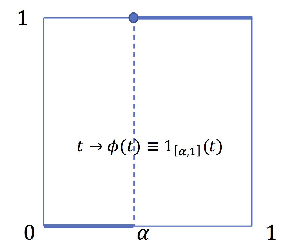
The first usual risk measure is the value at risk. VaR at \(\alpha>0\) is not a coherent measure because it is non convex. It is a distorsion measure associated with the distorsion function \(\phi(t)\equiv \mathrm{1}_{[\alpha,1]}(t)\) which is not a concave function. This property makes VaR a very poor and also "manipulable" risk measure (see below).
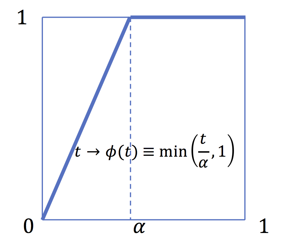
In contrast Expected Shortfall is a coherent risk measure. It is a distortion measure associated to the distortion function \(\phi(t)\equiv \min \left(\frac{t}{\alpha},1\right)\) which is a concave function.
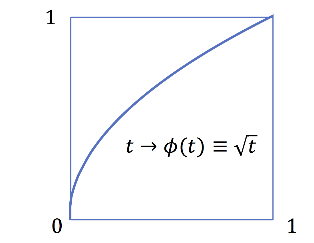
The risk measure \(\rho(\widetilde{w})\equiv \mathrm{ess-min}(\widetilde{w})=\underline{w}\) is a coherent risk measure. It entails an "infinite risk-aversion" or an infinite "pessimism" since it put the entire weight on the worst value.One can define"smoother" risk measures associated to smoother distorsion functions. For example "Proportional Hasard Rate" risk measures (PH) transform absolutely continuous distributions by multiplying the hasard rate by a constant \(\nu\). Noting \(\frac{dF}{dx}\equiv f\) and \(\frac{dG}{dx}\equiv g\) , the hasard rate are \(\frac{f}{F}\) and \(\frac{g}{G}\) . Namely if \(G\equiv \phi \circ F\), \(\frac{g}{G}=\frac{\phi'\circ F}{\phi \circ F} f\), so that \(\frac{\phi'\circ F}{\phi \circ F} f=\nu \frac{f}{F}\), that imply that we must have \(\frac{\phi'(t)}{\phi(t)}= \frac{\nu}{t}\), that is \(\phi(t)\equiv t^{\nu}\)
Value at Risk
VaR is a dsitorsion measure, associated to the distorsion
function \(t\rightarrow \mathrm{1}_{[\alpha,1]}(t)\) .It
is not a coherent risk measure since \(\phi\) is not
concave.
Expected Shortfall
ES is a distorsion measure associated to the distorsion
function \(t\rightarrow
\min\left(\frac{t}{\alpha},1\right)\). It is a coherent
risk measure (concave distorsion function)
Proportional hasard rate
PH is a distorsion measure associated to the distorsion
function \(t\rightarrow t^{\nu}\) where \(\nu < 1\). It
amounts to multiply the Hasard rate
\(\frac{1}{F}\frac{dF}{dx}\) by \(\nu\).
4.2 \(\mathrm{VaR}\) : a poor regulatory instrument
Most regulation rules impose financial institutions to hold reserves linked to VaR.
This is natural since the VaR is precisely defined as the stock of sure asset needed to lower the probability of failure less than \(\alpha\).
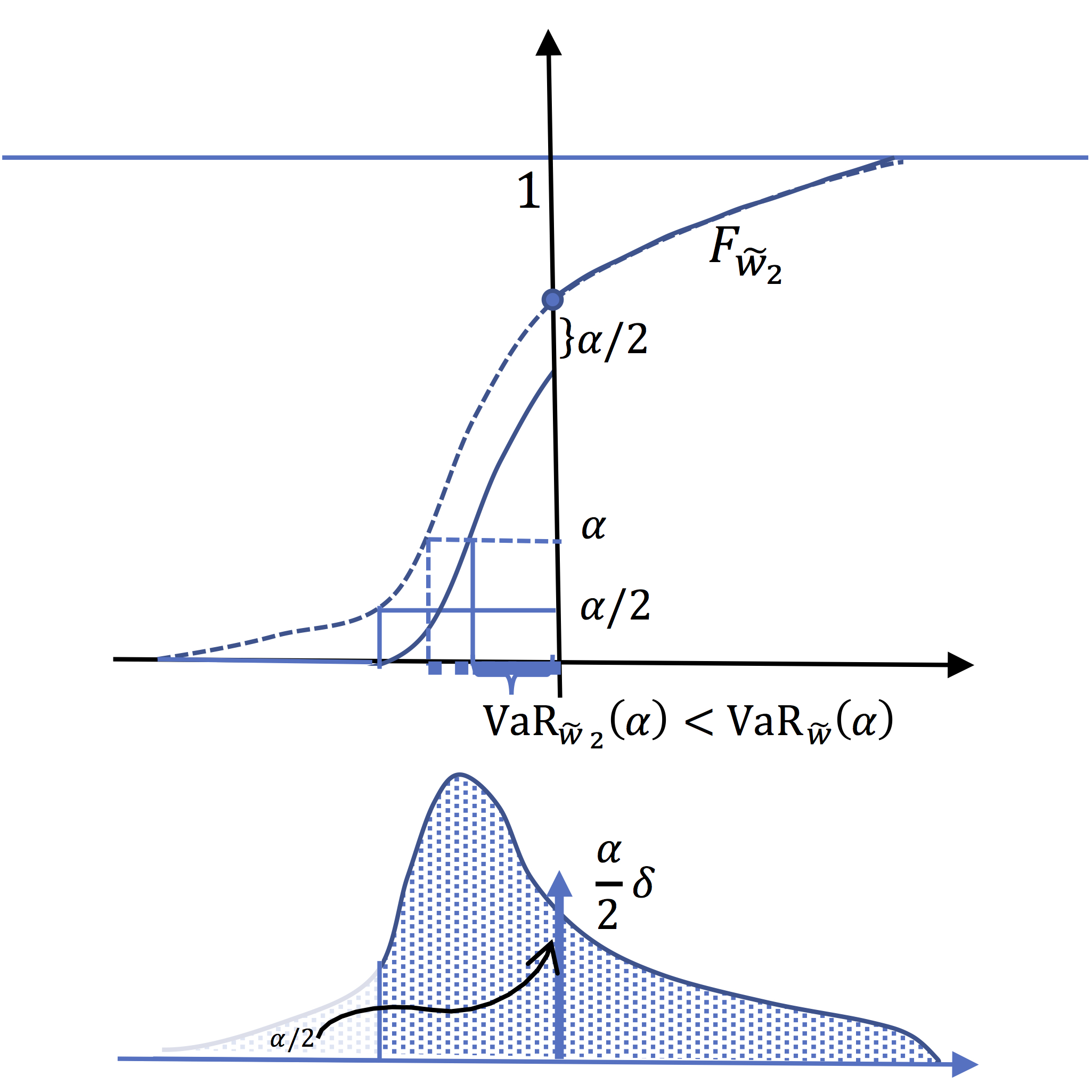
But the fact that VaR is not convex implies some bad properties concerning diversification of risk. Take for instance a regulation imposing a reserve equal to \(\mathrm{VaR}(\alpha)\). Let \(\widetilde{w}\) the income variable of a financial institution. And imagine that this firm creates two (100%) subsidiaries. The income of the first one is equal to \(\widetilde{w}_{1}\equiv \mathrm{1}_{[a,F^{-1}\left(\frac{\alpha}{2}\right)]}(\widetilde{w})\times \widetilde{w}\). The second has an income equal to :\(\widetilde{w}_{2}\equiv\mathrm{1}_{[F^{-1}\left(\frac{\alpha}{2}\right),b]}(\widetilde{w}) \times \widetilde{w}\)
In the following panels, is pictured the CDF of the two
subsidiaries. Tihs leads to conclude that \(\mathrm{VaR}_{\widetilde{w}_{1}}(\alpha)
+\mathrm{VaR}_{\widetilde{w}_{2}}(\alpha)<\mathrm{VaR}_{\widetilde{w}}(\alpha)\).
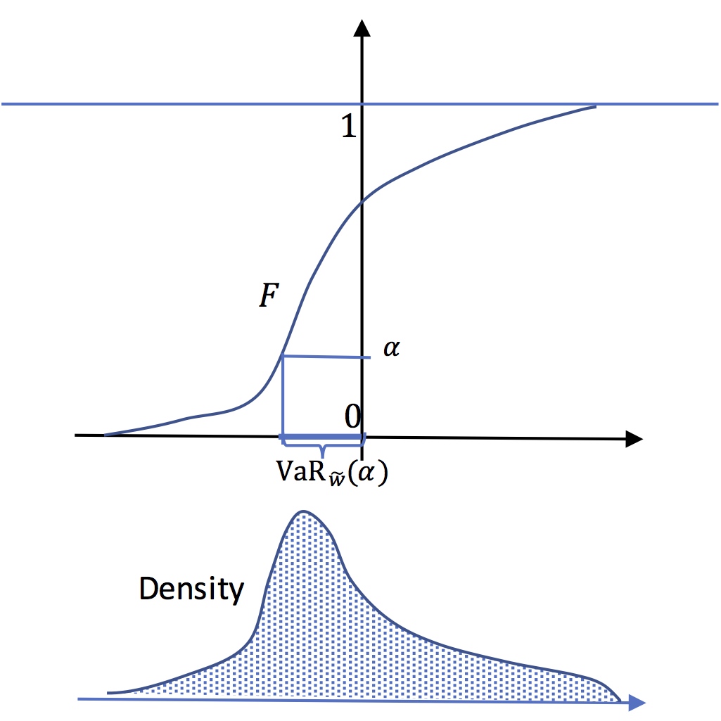
VaR of the firm
In this panel is represented \(F_{\widetilde{w}}\).
The Value at risk at level \(\alpha\) is positive.
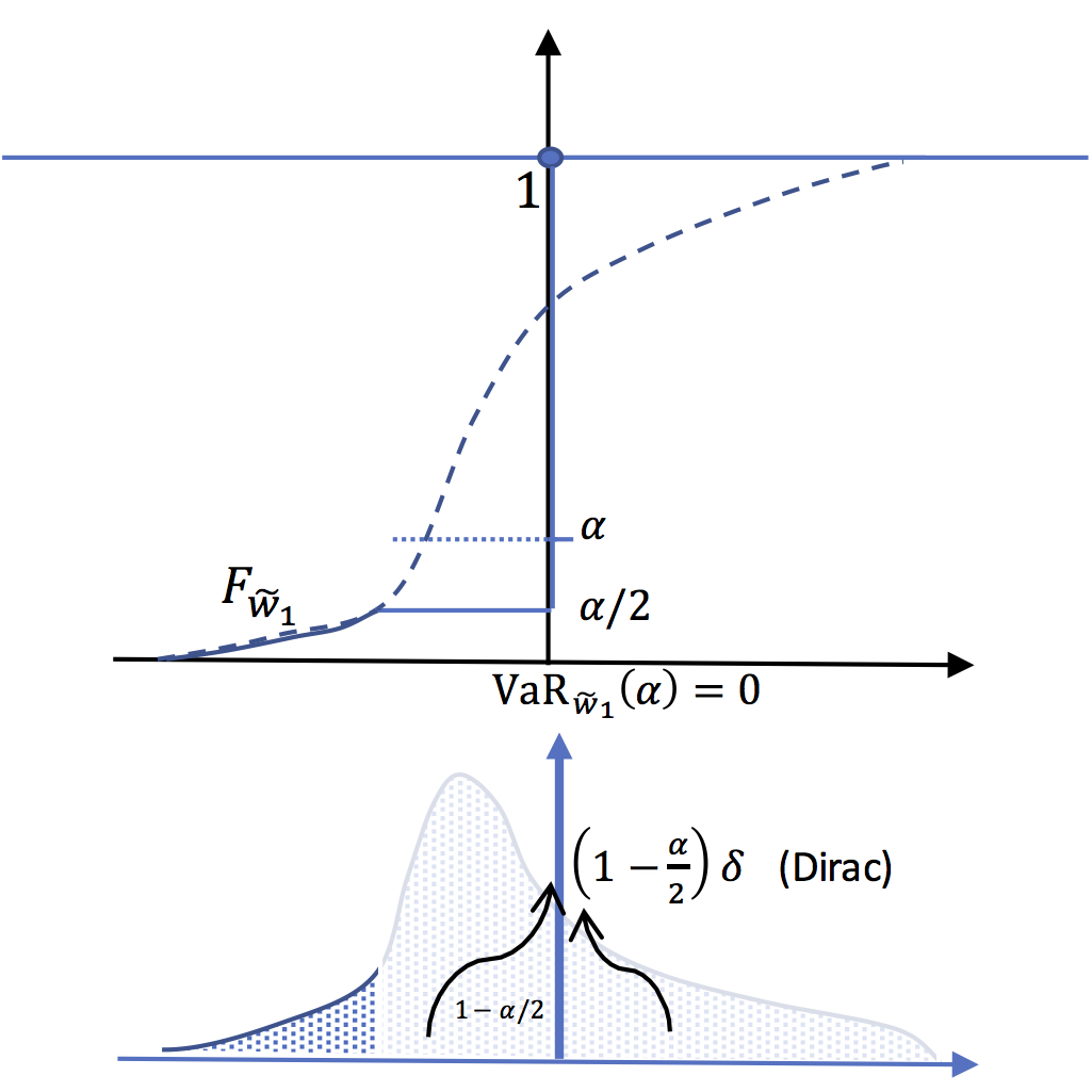
VaR of the first subsidiary is equal to zero :
In this panel is represented \(F_{\widetilde{w}_{1}}\).
All the mass above
\(F^{-1}_{\widetilde{w}}\left(\frac{\alpha}{2}\right)\),
i.e. exactly \(1-\frac{\alpha}{2}\), is
concentrated (Dirac mass) at 0. It follows that \(F^{-1}_{\widetilde{w}_{1}}\left(\alpha\right)=0\)
VaR of the second subsidiary is smaller than that of
the main firm :
In this panel is represented \(F_{\widetilde{w}_{2}}\).
We have (for \(x\leq0 \)), \(F_{\widetilde{w}_{2}}(x)=F_{\widetilde{w}}(x)-\frac{\alpha}{2}\)
This implies : \[F^{-1}_{\widetilde{w}_{2}}(t)=F^{-1}_{\widetilde{w}}(t+\frac{\alpha}{2})\]
So that The value at risk for this subsidiary is
equal to that of the firm at level \(\frac{3\alpha}{2}\)
which is less than \(\mathrm{VaR}_{\widetilde{w}}(\alpha)\)
Risk measures based on CDF, the expected utility approach
the preceding notions can also be defined by analyzing the integral of the distribution function or bi-cumulative.
5.1.Bicumulative function and second order stochastic dominance
Definition
We call bicumulative \(F_{\widetilde{w}}^{(2)}\) the function defined for \(x\in\left[a,b\right]\) by \[F_{\widetilde{w}}^{(2)}(x)=\int_{a}^{x}F_{\widetilde{w}}(y)dy\]
There is another writing of the bicumulative taht will be useful:
lemma
If \(\widetilde{w}\) is a random variable with support in \(\left]a,b\right[\) with right continuous non decreasing CDF \(F_{\widetilde{w}}\),then the bicumulative writes: \[F_{\widetilde{w}}^{(2)}(x)=\int_{a}^{x}F_{\widetilde{w}}(y)dy=xF_{\widetilde{w}}(x)-\int_{0}^{F_{\widetilde{w}}(x)}F_{\widetilde{w}}^{-1}(t)dt\]
We notice that \(F_{\widetilde{w}}^{(2)}(b)=b-\mathbb{E}(\widetilde{w})\). This above formula is well defined when \(a=-\infty\) and when \(\widetilde{w}\) has a finite expected value. For \(a>-\infty\) and \(b=+\infty\), this formula is obviously not well defined.In this case one takes the cumulative of \(1-F\) instead of those of \(F\)
This writing allows to put forward a remarkable relationship between the bicumulative function and the Lorenz function.
Proposition
Given a random variable with support in \(\left]a,b\right[\) we have : \[F_{\widetilde{w}}^{(2)}(x)=\max_{\alpha}\left[\alpha x-L_{\widetilde{w}}\left(\alpha\right)\right]\] \[L_{\widetilde{w}}\left(\alpha\right)=\max_{x}\left[x\alpha-F_{\widetilde{w}}^{(2)}\left(x\right)\right]\] (We say that the functions \(F_{\widetilde{w}}^{(2)} \) and \( L_{\widetilde{w}}\) are dual in the sense of Fenchel Moreau)
Indeed, Let \(\alpha^{*} \in \arg\max_{\alpha}\left[\alpha
x-L_{\widetilde{w}}\left(\alpha\right)\right]\).
We have \(L'_{\widetilde{w}-}(\alpha^{*})\leq x\leq
L'_{\widetilde{w}+}(\alpha^{*}) \)
That is \(F^{-1}(\alpha^{*})\leq x\leq F^{-1}(\alpha^{*}+)\).
Which implies \(\alpha^{*}=F(x)\)
and so : \(\max_{\alpha}\left[\alpha
x-L_{\widetilde{w}}\left(\alpha\right)\right]=
xF\left(x\right)-\int_{0}^{F(x)}F^{-1}\left(u\right)du=\int_{a}^{x}F(y)dy=F_{\widetilde{w}}^{(2)}(x)\)
The second equality is obtained in the same way.
Note that, in particular, we have \(F_{\widetilde{w}}^{(2)}(b)=\max_{\alpha}\left[\alpha b-L_{\widetilde{w}}\left(\alpha\right)\right]=b-E\left(\widetilde{w}\right)\)
From this we deduce the following result:
Proposition
Let Let two random variables \(\widetilde{v}\) and \(\widetilde{w}\) with support included in \(\left]a,b\right[\) with of the same expected value \(c\) \[\widetilde{w}\succsim\widetilde{v}\Longleftrightarrow\:\forall x,\:F_{\widetilde{w}}^{(2)}(x)\leq F_{\widetilde{v}}^{(2)}(x)\]
Indeed : \[\widetilde{w}\succsim\widetilde{v}\Longleftrightarrow\:\forall\alpha, L_{\widetilde{w}}\left(\alpha\right)\geq L_{\widetilde{v}}\left(\alpha\right)\Rightarrow\forall x,\alpha \alpha x-L_{\widetilde{w}}\left(\alpha\right)\leq\alpha x-L_{\widetilde{v}}\left(\alpha\right) \Rightarrow\forall x, \max_{\alpha}\left[\alpha x-L_{\widetilde{w}}\left(\alpha\right)\right]\leq\max_{\alpha}\left[\alpha x-L_{\widetilde{v}}\left(\alpha\right)\right]\]
Definition
Let two random variables \(\widetilde{v}\) and \(\widetilde{w}\) with support included in \(\left]a,b\right[\) . It is said that \(\widetilde{w}\) second-order stochastically dominates \(\widetilde{v}\), \(~\widetilde{w}\,\mathrm{SDD}\,\widetilde{v}\) , if \(\forall x,F_{\widetilde{w}}^{(2)}(x)\leq F_{\widetilde{v}}^{(2)}(x)\)
We can then conclude that for random variables with the same mean, second order stochastic dominance and mean preserved spread are equivallent concepts. The comparision of bicumulative functions or Lorenz function give the same information.
Proposition
Let \(\widetilde{v}\) and \(\widetilde{w}\) two random variables with support included in \(\left]a,b\right[\) and with the same expected value \(c\). \[\widetilde{w} \:\mathrm{SDD}\: \widetilde{v}\Longleftrightarrow\:\forall x,\:F_{\widetilde{w}}^{(2)}(x)\leq F_{\widetilde{v}}^{(2)}(x)\Longleftrightarrow\forall\alpha,L_{\widetilde{w}}(\alpha)\geq L_{\widetilde{v}}(\alpha)\Longleftrightarrow\widetilde{w}\succsim\widetilde{v}\]
5.2 Spectral indices and expected utility
We can construct preference criterions based on \(F\) and \(F^{2}\) in the same way as with quantile function. Let \(h\) an integrable function on \([a,b]\), and define a "spectral index" in a similar way as for the quantile function :
Definition
Given an integrable function \(h\) on \([a,b]\) one defines the spectral index associated to \(h\) by : \[U_{h}(\widetilde{w})\equiv -\int_{a}^{b}h(x)F(x)dx\]
We can first remark that if i \(h\) has a constant sign, for instance non negative, \(U_{h}\) is a criterion consistent with first order of stochastic dominance. Indeed :
Proposition
Let two random variables \(\widetilde{v}\) and \(\widetilde{w}\) with support included in \(\left]a,b\right[\). (i),(ii) and (iii) are equivalent :
(i) \(\widetilde{w}\:\mathrm{FSD}\:\widetilde{v}\)
(ii)\(\forall h\: \mathrm{non\: negative}\:, U_{h}(\widetilde{w})\geq U_{h}(\widetilde{v})\)
(iii)\(\forall x \in [a,b],\:F_{\widetilde{w}}(x)\leq F_{\widetilde{v}}(x)\)
Assume now that \(h\) is a non increasing right continuous function.\(-h\) is the cumulative function of a positive measure on \([a,b]\). Let \(d\ell\equiv -dh\) this measure. And rewrite \(U_{h}\) : \[-\int_{a}^{b}h(x)F(x)dx=\int_{a}^{b}\int_{a}^{x}d\ell(y)F(x)dx\] Or: \[U_{h}(\widetilde{w})=\int_{a}^{b}\int_{a}^{b}\mathbb{1}_{[a,x]}(y)d\ell(y)F(x)dx\] \[U_{h}(\widetilde{w})=\int_{a}^{b}\int_{a}^{b}\mathbb{1}_{[y,b]}(x)F(x)dxd\ell(y)\] That is \[U_{h}(\widetilde{w})=\int_{a}^{b}\{F^{(2)}(b)-F^{(2)}(y)\}d\ell(y)\] And finally : \[U_{h}(\widetilde{w})=(b-\mathbb{E}(\widetilde{w}))(h(a)-h(b))-\int_{a}^{b}F^{(2)}(y)d\ell(y)\] So that for two random variables with the same mean : \[U_{h}(\widetilde{w})-U_{h}(\widetilde{v})=\int_{a}^{b}(F_{\widetilde{v}}^{(2)}(y)-F_{\widetilde{w}}^{(2)}(y))d\ell(y)\] We can then state the following proposition :
Proposition
Let two random variables \(\widetilde{v}\) and \(\widetilde{w}\) with support included in \(\left[a,b\right]\) and with the same mean. (i),(ii) and (iii) are equivalent :
- (i) \(\widetilde{w}\:\mathrm{SSD}\:\widetilde{v} \)
- (ii)\(\forall x \in [a,b],\:F_{\widetilde{w}}^{(2)}(x)\leq F_{\widetilde{v}}^{(2)}(x)\)
- (iii)\( \forall h, \mathrm{non\: increasing,\:right\:continuous}\: U_{h}(\widetilde{w})\geq U_{h}(\widetilde{v})\)
Define then a so called "utility function" \(u\) (for any given
\(d\) in \([a,b]\) : \[[a,b]\rightarrow\mathbb{R},\:x\rightarrow
u(x)=\int_{d}^{x}h(y)dy\] We have : \[u'(x)\equiv h(x)\]
Definition
A utility function is a non decreasing function from \([a,b]\) to \(\mathbb{R}\) that captures the "satisfaction" achieved for a given level of income.
Then consider \(\mathbb{E}(u(\widetilde{w}))\equiv\int_{a}^{b}u(x)dF_\widetilde{w}(x)\) (where the integral is a Stieljes integral). A first computation gives : \[\mathbb{E}(u(\widetilde{w}))=\int_{a}^{b}u(x)dF(x)=\int_{a}^{b}\int_{d}^{x}h(y)dydF(x)\] or : \[\mathbb{E}(u(\widetilde{w}))=\int_{a}^{b}\left\{\int_{a}^{d}\mathbb{-1}_{[x,d]}(y)h(y)dy\right\}dF(x)+\int_{a}^{b}\left\{\int_{d}^{b}\mathbb{1}_{[d,x]}(y)h(y)dy\right\}dF(x)\] or \[\mathbb{E}(u(\widetilde{w}))=\int_{a}^{d}\left\{\int_{a}^{b}\mathbb{-1}_{[a,y]}(x)dF(x)\right\}h(y)dy+\int_{d}^{b}\left\{\int_{a}^{b}\mathbb{1}_{[y,b]}(x)dF(x)\right\}h(y)dy\] that is \[\mathbb{E}(u(\widetilde{w}))=\int_{a}^{d}\left\{F(a)-F(y)\right\}h(y)dy+\int_{d}^{b}\left\{F(b)-F(y)\right\}h(y)dy\] that is \[\mathbb{E}(u(\widetilde{w}))=u(b)-\int_{a}^{b}F(y)h(y)dy=u(b)+U_{h}(\widetilde{w})\]
This simple computation means that the criterion \(U_{h}\) gives the same preference criterion as \(\mathbb{E}(u(.)\) where \(u\) is an integral of \(h\). We can the define the Expected Utility Assumption :
Definition
We say that the decision is based on expected utility if it exits a real increasing function \(u\), such that for all random variable of income \(\widetilde{w}\) and \(\widetilde{v}\) , \(\widetilde{w}\) is preferred to \(\widetilde{v}\) if and only if \[\mathbb{E}\left[u\left(\widetilde{w}\right)\right]\geq\mathbb{E}\left[u\left(\widetilde{v}\right)\right]\]
As in the previuous section, we conclude that a decisionmaker that prefers high income would use a spectral index \(U_{h}\) with a non negative \(h\). If moreover he prefers concentrated distributions, then he would use positive, non increasing right contiunuous function \(h\). This amounts then to use an "expected utility" citerion with a utility function \(u\) increasing and concave.
5.3. Risk aversion in the expected utility approach
In the expected utility approach, we say that the decision maker is risk-averse if for all \(w_{0}\in \mathbb{R}\) and all pure risk \(\widetilde{x}\) such that \(\mathbb{E}(\widetilde{x})=0\), he prefers \(w_{0}\) to \(w_{0}+\widetilde{x}\). This definition amounts to assume that the decision maker prefers an income infinitely concentrated on the mean to any dispersion around it. By noting \(\widetilde{w}\equiv w_{0}+\widetilde{x}\) this amounts to assume that \(\mathbb{E}(u(\widetilde{w}))\leq u(\mathbb{E}(\widetilde{w})\). This means obviously that \(u\) must be concave. As we have assumed that \(u\) is non decreasing, he moreover prefers high income to low ones.
Proposition
In the expected utility approach, risk-aversion is equivallent to \(u\) is a concave function
Summary and final remarks
To summarize, there is somme symmetry (in fact duality) between the CDF or expected utility approach (primal) and the quantile or distorsion criterion approach (dual or Yaari's). Risk aversion, in both approaches, simply means that the decision maker prefers concentrated distrubutions to spread ones. That implies that the utility function (primal approach) and the distorsion function (dual) are concave.
Quantile approach
- \(\widetilde{w}\: \mathrm{FSD}\:\widetilde{v}\)
\(\Longleftrightarrow F_{\widetilde{w}}^{-1}(\alpha) \geq F_{\widetilde{v}}^{-1}(\alpha)\)
\(\Longleftrightarrow \forall \alpha,\:\mathrm{VaR}_{\widetilde{w}}(\alpha) \leq \mathrm{VaR}_{\widetilde{v}}(\alpha)\)
\(\Longleftrightarrow \forall \varphi \geq 0, R_{\varphi}(\widetilde{w})\geq R_{\varphi}(\widetilde{v})\) \(\Longleftrightarrow \forall \phi \: \mathrm{non \: decreasing}, S_{\phi}(\widetilde{w})\geq S_{\phi}(\widetilde{v})\)
- \(\widetilde{w}\: \mathrm{SSD}\:\widetilde{v}\)
\(\Longleftrightarrow L_{\widetilde{w}}(\alpha) \geq L_{\widetilde{v}}(\alpha)\)
\(\Longleftrightarrow \forall \alpha,\:\mathrm{ES}_{\widetilde{w}}(\alpha) \leq \mathrm{ES}_{\widetilde{v}}(\alpha)\)
\(\Longleftrightarrow \forall \varphi \mathrm{non \: begative \: non \: increasing}, R_{\varphi}(\widetilde{w})\geq R_{\varphi}(\widetilde{v})\) \(\Longleftrightarrow \forall \phi \: \mathrm{non\:decreasinq\:concave}, S_{\phi}(\widetilde{w})\geq S_{\phi}(\widetilde{v})\)
CDF approach
\(\mathrm{integrate \:by\:part}\: U_{h}(\widetilde{w})\) gives:
\(\int_{a}^{b}u(x)dF_{\widetilde{w}}(x)\equiv\mathbb{E}(u(\widetilde{w})\)
- \(\widetilde{w}\: \mathrm{FSD}\:\widetilde{v}\)
\(\Longleftrightarrow F_{\widetilde{w}}(x) \leq F_{\widetilde{v}}(x)\)
\(\Longleftrightarrow \forall h \geq 0, U_{h}(\widetilde{w})\geq U_{h}(\widetilde{v})\) \(\Longleftrightarrow \forall u \: \mathrm{non \: decreasing}, \mathbb{E}(u(\widetilde{w}))\geq \mathbb{E}(u(\widetilde{v}))\)
- \(\widetilde{w}\: \mathrm{SSD}\:\widetilde{v}\)
\(\Longleftrightarrow F_{\widetilde{w}}^{2}(x) \leq F_{\widetilde{v}}^{2}(x)\)
\(\Longleftrightarrow \forall h \mathrm{non \: begative \: non \: increasing}, U_{\varphi}(\widetilde{w})\geq U_{\varphi}(\widetilde{v})\) \(\Longleftrightarrow \forall u \: \mathrm{non\:decreasinq\:concave}, \mathbb{E}u(\widetilde{w}))\geq \mathbb{E}((\widetilde{v}))\)
Remark
The quantile approach is scale independent : when income is multiplied by any positive number, the criterions are multiplied by the same constant. It is not the case for Expected utility approach. Assume for instance that \(u\) is concave with \(u(0)=0\). Then \(\mathbb{E}\left[u\left(\lambda \widetilde{w}\right)\right]\leq \lambda \mathbb{E}\left[u\left(\widetilde{w}\right)\right]\).This means that expected utility criterion is scale dependent. In particular, in the expected utility approach, risk aversion (concavity of \(u\)) can vary with the level of income.
Some other results : mutualization and diversification
The previous resuts are quite useful to proove some results
related to diversification or mutualization of risk. The idea is
quite very simple. Assume for instance \(n\) individuals exposed
to a risk in income. Income of individual \(i\) is a random
variable \(\widetilde{w}_{i}\) on \(]a,b[\). Assume that these
variable are identically distributed (but not necessary
independent). Let \(F\) the joint CDF :
\(F(x_{1},x_{2},...,x_{n})=\Pr{\land_{i=1}^{n}\widetilde{w}_{i}\leq
x_{i}}\).The marginal \(F_{\widetilde{w}_{i}}\) is defined by
\(F_{\widetilde{w}_{i}}(x)= F(b,b,...x_{i}=x,...,b)\). Assuming
that they are identically distributed means that the marginals are
the same. The mutualization principle says that \(\frac{1}{n}
\sum_{i=1}^{n} \widetilde{w}_{i}\) is less risky (i.e more
concentrated) than any original variable \(\widetilde{w}_{i}\).In
fact one can even proove a more general result :
Proposition
Let \(n\) random income \(\widetilde{w}_{i}, i=1...n\) identically distributed with support in \(]a,b[\). \[\forall \lambda_{i}\geq 0, i=1...n, \: \sum_{i=1}^{n}\lambda_{i}=1,\: \forall j, \: \sum_{i=1}^{n}\lambda_{i}\widetilde{w}_{i} \succsim \widetilde{w}_{j}\]
The proof is quite simple : firts of all \( \sum_{i=1}^{n}\lambda_{i}\widetilde{w}_{i}\) and \(\widetilde{w}_{i}\) have the same mean. So that to proove that the first one is less risky, it is sufficient to show that any risk-averse decision maker prefers the first one. So take a concave function \(u\) and compute \(\mathbb{E}\left[u\left(\sum_{i=1}^{n}\lambda_{i}\widetilde{w}_{i}\right)\right]\). By concavity of \(u\), this is larger than \(\mathbb{E}\left[\sum_{i=1}^{n}\lambda_{i}u\left(\widetilde{w}_{i}\right)\right]\), which is equal to \(\sum_{i=1}^{n}\lambda_{i}\mathbb{E}\left[u\left(\widetilde{w}_{i}\right)\right]\).As all icommes have the same distribution, all the \(\mathbb{E}\left[u\left(\widetilde{w}_{i}\right)\right]\) are identical, so that this expression reduces (for any \(j\)) to \(\mathbb{E}\left[u\left(\widetilde{w}_{j}\right)\right]\). Notice that this rsult is also valid for non bounded variables provided that they have a finite mean.
We have also an important result in the case of independent risks : the risk of the mutualized income reduces when \(n\) increases. That is the basis of "law of large numbers".
Proposition
Let a sequence random income \(\widetilde{w}_{i}, i=1...n...\) identically distributed and independent, with \(\mathbb{E}\widetilde{w}_{i}<\infty\). Then, if \(p\leq q\), \(\frac{1}{p}\sum_{i=1}^{p}\widetilde{w}_{i}\) is a mean preserving spread (less concentrated) of (than) \(\frac{1}{q}\sum_{i=1}^{q}\widetilde{w}_{i}\).That is : \[p\leq q \Longrightarrow \frac{1}{q}\sum_{i=1}^{q}\widetilde{w}_{i} \succsim \frac{1}{p}\sum_{i=1}^{p}\widetilde{w}_{i}\]
The proof is done by recurrence. It is obviously true (by the
previous proposition) for \(p=1\) and \(q=2\). Assume it is true
for \(p\leq q \leq n-1\).Let \(S_{n-1}^{i}\equiv
\frac{1}{n-1}\sum_{j\neq i,j\leq n}\widetilde{w}_{j}\). The
variables \(S_{n-1}^{i},i=1,...n,\) are identically distributed.
And we have
\(\frac{1}{n}\sum_{i=1}^{n}S_{n-1}^{i}=\frac{1}{n}\sum_{j=1}^{n}\widetilde{w}_{j}\).
So, we deduce by the previuous proposition that
\(\frac{1}{n}\sum_{j=1}^{n}\widetilde{w}_{j}\) is less risky than
each \(S_{n-1}^{i}\). Which gives the result.
Notice that this result is valid for variables with finite means.
It is NOT true for variables distributed for instance according to
a Cauchy distribution.Indeed in that case
\(\frac{1}{n}\sum_{i=1}^{n}\widetilde{w}_{i}\) has the same
distribution as each \(\widetilde{w}_{i}\)!.This result can be
generalized to symmetrical distributed variables.
Diversification
These results are the basis of the diversification principle.
Assume for instance you have \(K\) assets with random returns
\(\widetilde{x}_{i}\). One euro invested on asset \(i\) will give
\(\widetilde{x}_{i}\) euros next period. Assume that these assets
are identically distributed. Then diversificating the portfolio,
that is investing \(\lambda_{i}\) euros in asset \(i\) with
\(\sum_{i=1}{n}\)\lambda_{i}=1\) gives a less risky return than
investing on only one of the original assets.
This is the diversification principle that says that you reduce risk when you don not put all your eggs in the same basket.